Step 7: Construct Climate Projections
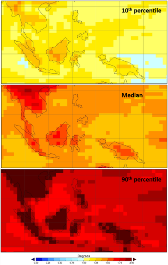
Climate projections must include all selected model simulations in your computations or analyses to fully capture the distribution of the projected changes. The mean or median consensus of the projections, and the plausible range of the whole selected model ensemble, could also be generated. This is typically represented by the 10th and 90th percentile of the changes or by the maximum and minimum values of the changes.
For example, you may have decided in step 6 to analyze the outputs of 40 GCMs to calculate projected change in annual rainfall for 2030–2060, relative to 1980–2010. In this case, you need to calculate the projected change for each of the 40 GCMs. Subsequently, subject to the project context, you may need to show each individual result, or you may need to summarize the results of the 40-model ensemble by calculating the 10th, 50th (median), and 90th percentile of these 40 projected changes.
Climate projections may be constructed in a number of ways, depending on the application. These could be in a form of projected change in a given climate variable in the future relative to a baseline or as a long-term trend into the future.
Climate change fields of relevant variables
The most common case is to produce the change signals for the variables for each of the selected model data. The changes are expressed as the differences in future climate relative to the present (baseline). This involves calculating averages over a period of time for both future and historical periods, then subtracting the historical value from the future value. For example, if for a given grid the modelled temperature average for 2020–2050 is 29 °C while that of the historical periods is 28 °C, then the modelled projected change for that grid is 1 °C. This procedure is completed for all the model grid boxes under the region of interest. It is important to select a sufficiently long time period for averaging to ensure the change signal is not influenced by natural variation.
With respect to the presentation of results (step 10), the projected change from each individual model can be displayed independently. Alternatively, you may display the median or mean along with some measure of spread, such as the 10th and 90th percentile, of various model projections (as in this figure).
Long-term trends into the future
Another common case is to provide broad information of the climate change signal over time. This could be constructed by plotting time series of the selected variables from the historical period into the future.
The plot can be either for a location or averaged over a region depending on the focus and/or methodology of the study.
Applying smoothing, such as an 11-year moving average, can more clearly show the climate change signal by removing some of the shorter-term variability that might otherwise obscure the signal. As with the mean changes in climate, some measure of the median/mean projection along with the 10th and 90th percentile values of all the projections can be used to summarize the range. Displaying the projections of multiple climate models in the time series allows the end user to better understand the range of possible futures
CASE STUDY EXAMPLES


