Step 5: Collect and Evaluate Climate Model Data
Climate projections data are usually generated from climate model outputs. With so many climate model outputs and datasets available, it is not possible to look at all the raw model data that are available. It is essential to identify your requirements so you can collect appropriate climate projections data about the future climate.
The closer the model simulation is to the observed climate, the closer the modelled climate change response of the simulation will be to the real-world response, and the higher the confidence rating in your projections.
Pacific Climate Futures is a valuable online resource for accessing and evaluating regional climate projections for the western tropical Pacific. The activities outlined in this step are for the most part based on use (access and application) of this tool.
Key activities
- Identify the baseline period
- Identify the scenarios of interest
- Decide which climate models to use
- Create the application-ready dataset
- Evaluate the model data
Identify the baseline period
Climate projections describe ranges of possible change into the future relative to a ‘baseline’ period in the past. The climate has changed in the past, so the choice of baseline is important.
Some information is given relative to the ‘pre-industrial era’, which means before industry ramped up in the 1800s. For example, the global average temperature is around 1 °C warmer than pre-industrial times. However, most climate projections are given relative to a recent baseline (a 20- or 30-year period in the recent past), so that we can understand the future relative to what we have recently experienced. For example, PACCSAP refers to 1986–2005 as the baseline period. This baseline is also used by the Intergovernmental Panel on Climate Change (IPCC) for its assessment reports.
Identify the scenarios of interest
We can’t predict how greenhouse gas and aerosol emissions will continue in the future, or what their atmospheric concentrations will be. However, this is important information for generating climate projections. To overcome this problem, a set of scenarios have been developed that describe conditions for a range of emissions and concentrations. These scenarios are called representative concentration pathways (RCPs). There are four RCPS: RCP2.6 (lowest), RCP4.5, RCP6 and RCP8.5 (highest). Because of natural variability in the climate, the results from the different scenarios are quite similar to 2030. However, after this time, the higher the emissions, the more climate change you see by 2100. To show the ‘worst case’ you might only consider the highest scenario, while a ‘best case’ would consider one of the lower scenarios.

IMPORTANT: Be careful with the choice of emissions scenarios (that is, not using enough or using the wrong one for the analysis). Using inputs that are too specific could mean that not all future climate possibilities are taken into consideration, which could result in inappropriate or ‘mal-adaptive’ responses. For example, considering only a best-case (low emissions) scenario for temperature change may be overly optimistic and thereby underestimate the associated risks of increasing incidence of temperature extremes with consequent impacts on human health, water and food security. Similarly, considering only a worst-case (high emissions) scenario for rainfall may result in the commitment of valuable but otherwise limited resources to unnecessary adaptation activities, such as building reservoirs or desalination plants to accommodate a change in water supply that does not eventuate. Including the best and worst cases provides a range of possible climate futures.
Decide which climate models to use
All climate models simulate the climate a little differently due to how they are set up and how they work. For this reason, it is important to never just look at one model. It is generally a good idea to reject models if they are completely unsuitable (perhaps due to inherent bias or other design limitations in the model), but then compare all the rest of the acceptable models to make projections (e.g. PACCSAP looked at 27 CMIP5 models and rejected three as unsuitable but then used the rest). Projections from technical forms of downscaling (statistical or dynamical models) may also be available.
If a change in the average for just one variable over the nation is needed, use model ranges from reports. If using daily or monthly data and more than one variable, choose a set of representative models using the Pacific Climate Futures tool.
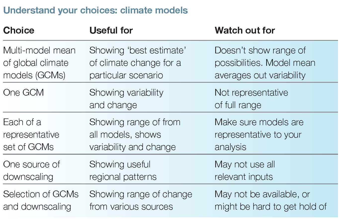
IMPORTANT: Do not just look at one climate model output – models give different estimates of change, and just looking at one model won’t give the range indicated by the climate models. Instead, use a representative set.
Create the application-ready dataset
Global climate models have a coarse spatial resolution (typically 100–250 km grid box) and contain biases or offsets compared to observations, so their outputs don’t look exactly like observations. Model outputs generally can’t be used directly – additional steps must be taken to make a future dataset that is locally relevant and has no biases. The simplest way to do this is by scaling observations. Various technical downscaling methods exist that can also achieve these goals, as well as potentially showing more information about regional climate change.
Scaling observations is also known as the ‘delta’, ‘perturbation’ or ‘change factor’ method. Scaling involves applying the projected climate change to the observations to make a hypothetical dataset of the future conditions. The observations can be scaled up or down by the projected average change, called mean scaling. Observations can be scaled using a different scaling for different values (with scaling factors calculated from model outputs), which is an example of complex scaling. Other complex scaling methods exist, including ‘weather generators’.
Mean scaling is the simplest method. To do this:
- Take a suitable observed dataset.
- Collate a range of suitable change factors from climate projections.
- Apply the change factor to the observed dataset to make the future dataset. The change factor is applied using an addition for variables such as temperature, or as a multiplication for variables such as rainfall.
Scaling observations using global climate model projections is the default option for producing locally-relevant, application-ready datasets. It is important to collect a representative set of scaling factors to cover the changes of interest (showing the range from sets of relevant models for each emission scenario). If complex or technical downscaling has been done for the area in question, and the downscaled outputs are available to be used, these outputs can be used instead or as well.
Evaluate the model data
Model data evaluation may simply be a case of comparing the modelled climate against the observed climate. You might include the long-term average, standard deviation (which represents year-to-year variability) or annual or seasonal cycle of the relevant climate variables (e.g. temperature and rainfall).
When resources permit, it is also useful to assess how the model represents the observed characteristics of large-scale climate features such the El Niño–Southern Oscillation or the major rainfall bands called the Inter-Tropical Convergence Zone (ITCZ) and the South Pacific Convergence Zone (SPCZ), or how the model reproduces the observed relationship between climate variables (e.g. rainfall) and large-scale climate features (e.g. ITCZ or SPCZ).
IMPORTANT: Use the simplest dataset available that covers the required range of relevant climate variables and projections.