Define Project Inclusions and Exclusions
In many cases, project resources are limited, so it is essential to be clear about your focus.
You (with your stakeholders or users) decide what to include and what to exclude in your project. Considerations include:
- boundaries (physical and non-physical)
- climate variables
- type of climate data
- spatial considerations
- temporal considerations
- outputs or products.
Boundaries (physical and non-physical)
Physical boundaries could be administrative (e.g. province, district), environmental (e.g. river basin, catchment), or a service system (e.g. urban water supply system). Non-physical system boundaries relate to things like the social and economic dynamics of the community, regulation, and institutional structures whose spatial units may range from local (e.g. households or villages) to national level. These boundaries will inform the spatial resolution of climate information that is required.
Climate variables
The variables to be included will vary depending on the project purpose and context.
Your project may need common climate variables such as temperature, solar radiation and rainfall, and/or derived variables such as extreme rainfall, Standardized Precipitation Index (SPI, a measure of meteorological drought) and the annual number of hot days or cool days (which measure extreme temperature events).
Derived variables are calculated from common climate variables. For example, extreme rainfall may be calculated from daily rainfall data, while monthly rainfall data is used to calculate SPI.
In some cases, a derived index such as the Southern Oscillation Index (SOI) is needed for identifying possible changes in important large-scale climatic variations. This index gives an indication of the El Niño and La Niña events in the Pacific Ocean, which influence rainfall variability over much of the South East Asia region. This index is calculated using monthly mean sea-level pressure differences between Darwin and Tahiti.
Type of climate data
Climate data may be collected from observations or generated from climate models. Observed climate information is generally used to tell us about the past and present, while modelled data is generally used when developing information about the future.
Observed climate data may be used to:
- evaluate climate model data prior to constructing climate model-based projections (step 5)
- conduct climate model bias-correction (step 9) before their use in an impact model
- establish a baseline condition
- analyze current and historical impacts or trends through, for instance, a detection and attribution study
- calibrate an impact model.
Modelled climate data may be used to:
- develop projected changes in a given climate variable in a given future period relative to that in a given historical baseline period (step 7)
- project long-term trends by constructing a time series plot of a given modelled climate variable from the 20th to the 21st century (step 7).
You may need to use observed climate data, modelled climate data or both.
Spatial considerations
The first spatial consideration is the spatial unit of analysis. You need to decide whether your analysis level is, for instance, for the bulk of the province, at the district level within the province, or at another level or specific location(s).
The unit of analysis will determine if your data needs to be station-based or gridded. Station-based data may be useful for a single or several locations, while analysis of a region or a country may be better served using gridded data.
The unit of analysis will also determine the spatial resolution of climate information that needs to be considered.
If you want to assess the province as a whole region and the province’s climate is relatively homogenous, it may be enough to consider coarse climate data from a global climate model (GCM) simulation if GCM data are all you have. But if the province is in a mountainous region (e.g. Nepal) or on a small island (e.g. Bali) whose climate varies spatially, then you may need to use finer scale model data. Similarly, if your analysis is for the sub-district level within each of the districts in the province, and their climate is heterogeneous, then you may need to use finer-scale climate data produced by downscaling simulations if possible.
You may need to redefine the spatial resolution when you are establishing the project context (step 1), or when you are collecting your observed (step 2) or modelled (step 4) climate data.
It is important to note that:
- availability of observed climate data with high spatial resolution varies with country and region.
- simulations from GCMs are typically at the resolution of a 60–410 km grid box. For small islands or regions with complex topography or heterogeneous climate, this resolution may be too coarse to adequately capture local climate. To address this, high-resolution regional climate models are often used to provide more detailed climate simulation at resolutions of 10 km or less if possible.
Temporal considerations
There are a number of time-based considerations when scoping your project, including:
- time period (how long your baseline and projection periods should be)
- future time horizon (the period of future time your analysis needs to be valid for)
- temporal resolution (e.g. annual, monthly, daily)
You may need to define both the baseline (or historical) and future time period for your project, depending on your objective.
If your objective is to develop future climate projections relative to the present (baseline), then the time period of data should be aligned with the time horizon (described below).
The World Meteorological Organization (WMO) suggests a 30-year baseline period, but the decision depends on your project context. In addition to data availability and quality, you should consider if the baseline time period meets the following criteria[1]:
- Is it representative of the present-day or recent average climate in the study region?
- Is it long enough to encompass a range of natural climatic variations?
- Is it consistent with or readily comparable to baseline climatologies used in other assessments?
If your objective is to analyze long-term trends based on observed climate data, then the time period must be long enough to capture the key modes of natural variability. Such variability occurs on timescales of months, seasons, years, decades, and multi-decades. It is driven by major climate influences such as the El Niño–Southern Oscillation and the Interdecadal Pacific Oscillation. In this context, a 30-year period may not be sufficient.
If your objective is to use observed climate data to calibrate a given impact model, then the time period must be long enough (> 30 years, if possible) to capture natural variability. Due to data availability, many cases usually use observed data for around 20–30 years for calibrating and evaluating impact model.
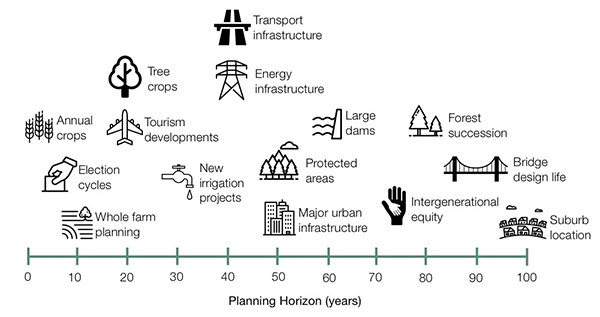
The time horizon for your project will depend largely on the planning horizon for the sector your climate information is being developed for. Planning horizons may extend from 15–20 years for project or program loan repayment, through to 30–120 years for the design service lifetime of a water supply system (depending on assumptions of a static or dynamic population as well as pipe materials). Other planning horizon examples are provided in this figure.[2]
You need to decide whether the temporal resolution will be on an annual, seasonal, monthly, daily, or another timescale. In some cases, annual climate data may suffice (e.g. for mapping projected change in annual rainfall across a country) but in others, monthly data could be needed (e.g. for computing SPI as a measure of drought). In other situations, daily data could be essential (e.g. for computing the annual number of hot days or cool days as a measure for extreme temperature events).
It is important to note that the shorter the temporal scale (e.g. sub-hourly, hourly and daily) for observed climate data, the less likely the data is available.
You should also remember that climate model simulations are designed to indicate trends or projected climatological change over decades or longer time periods. They are not designed to simulate specific values for given climate variables for specific days, as you would expect from a much shorter-term weather forecast.
While a climate model may do a good job at simulating a longer timescale (e.g. monthly or annual climatology), caution is needed when dealing with data at a finer timescale (e.g. daily or hourly). Even if daily climate model simulations for 100 years in the future are available you should not treat these daily model data as observed daily data. This is very important to note, especially if you need time series of climate model data for use in an impact assessment model. In most cases, you need to do an additional step (e.g. bias correction, step 9) before you can use climate model time series in an impact model. This is also important to note if your objective is to project hourly extreme rainfall, for instance.
Outputs or products
You should consider what outputs or products will best suit your objectives, as this will guide you on how to communicate or report results (step 10).
For example, if your purpose is to develop climate projections information, is that information best delivered in the form of a database, summary table, maps, figure, report, or another format?
[1] IPCC-TGICA. 2007. General Guidelines on the Use of Scenario Data for Climate Impact and Adaptation Assessment. Version 2. Prepared by T.R. Carter on behalf of the Intergovernmental Panel on Climate Change, Task group on data and Scenario Support for Impact and Climate Assessment, 66 pp.
[2] Modified from: Jones R, McInnes K. 2004. A scoping study on impact and adaptation strategies for climate change in Victoria. CSIRO Atmospheric Research, Melbourne, Australia: Report to the Greenhouse Unit of the Victorian Department of Sustainability and Environment.